- MATLAB 100%
| Filename | Latest commit message | Latest commit date |
|---|---|---|
| +MTracer | ||
| assets | ||
| external | ||
| release | ||
| scripts | ||
| .gitignore | ||
| MTracer.mlapp | ||
| MTracer.prj | ||
| MTracerTrace.m | ||
| MTracerVM.m | ||
| README.md | ||
| ReleaseNote.txt | ||

MTracer
A MATLAB app to visualize and correct tissue motions in Neuropixels recordings, and to curate spike clusters in the context of the tissue motion.
Publications using MTracer:
-
JE Chung, KK Sellers, MK Leonard, L Gwilliams, D Xu, ME Dougherty, V Kharazia, SL Metzger, M Welkenhuysen, B Dutta, EF Chang. High-density single-unit human cortical recordings using the Neuropixels probe. Neuron, 2022. (Link)
-
MK Leonard, L Gwilliams, KK Sellers, JE Chung, D Xu, G Mischler, N Mesgarani, M Welkenhuysen, B Dutta, EF Chang. Large-scale single-neuron speech sound encoding across the depth of human cortex. Nature, 2023. (Link)
-
D Xu, JE Chung, AB Silva, SL Metzger, QR Greicius, Y Zhang, MK Leonard, EF Chang. Human precentral gyrus neurons link speech sequences from listening to speaking. bioRxiv, 2024. (Link)
Installation
There are two ways to install MTracer:
1. Add to Path (Recommended)
- Clone or download this repository
- Add the repository folder to your MATLAB path
- In MATLAB, Home -> Set Path -> Add with Subfolders -> Select the repository folder
- Or run
addpath(genpath('path_to_mtracer'))in the MATLAB command window
- This will also include the three external dependencies in the
externalfolder:ManyFunMatlabneuropixel-utilsnpy-matlab
2. App Installer
- Double-click the
\release\MTracer.mlappinstallfile to install it in MATLAB - The app will appear in the MATLAB Apps tab
- Note that installing with the app installer will not give you access to the source code of the app
Compatibility
- Requires MATLAB 2021a or later
- To read Kilosort 4 results, Python must be available to MATLAB
Run the App
For most users
Run "MTracer" from the MATLAB command window.
Tip: you can save this command to the Favorites tab for quick access.
As an object (for advanced users)
mtracer = MTracerVM;
Maps Window
The Maps Window is the main visualization interface of MTracer, implemented as a LayeredFigure that manages multiple plot layers. Each layer can be toggled independently for different use cases:
- Focus Layer: Crosshair highlighting the currently selected point on the maps.
- LFP Layer: Displays low-passed local field potential data as a heatmap, showing the continuous voltage signals across channels over time.
- AP Layer: Shows action potential (spike) voltage traces around the focus when requested by pressing 'v'.
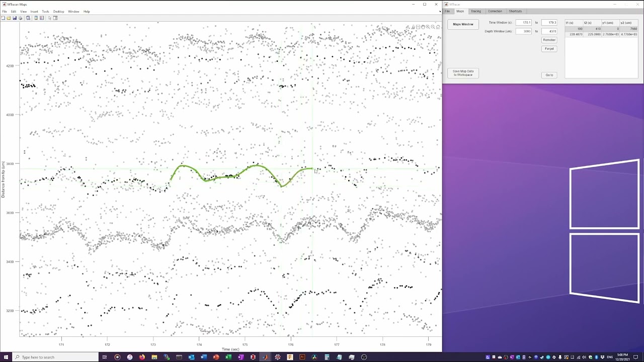
- Drift Map Layer: Visualizes individual spikes from Kilosort's "drift map" as dots, with their y-positions corresponding to detection locations.
- Traces Layer: Displays the smooth tissue motion tracking traces.
- Trace Anchors Layer: Displays anchor points the user created for the tissue motion tracking traces.
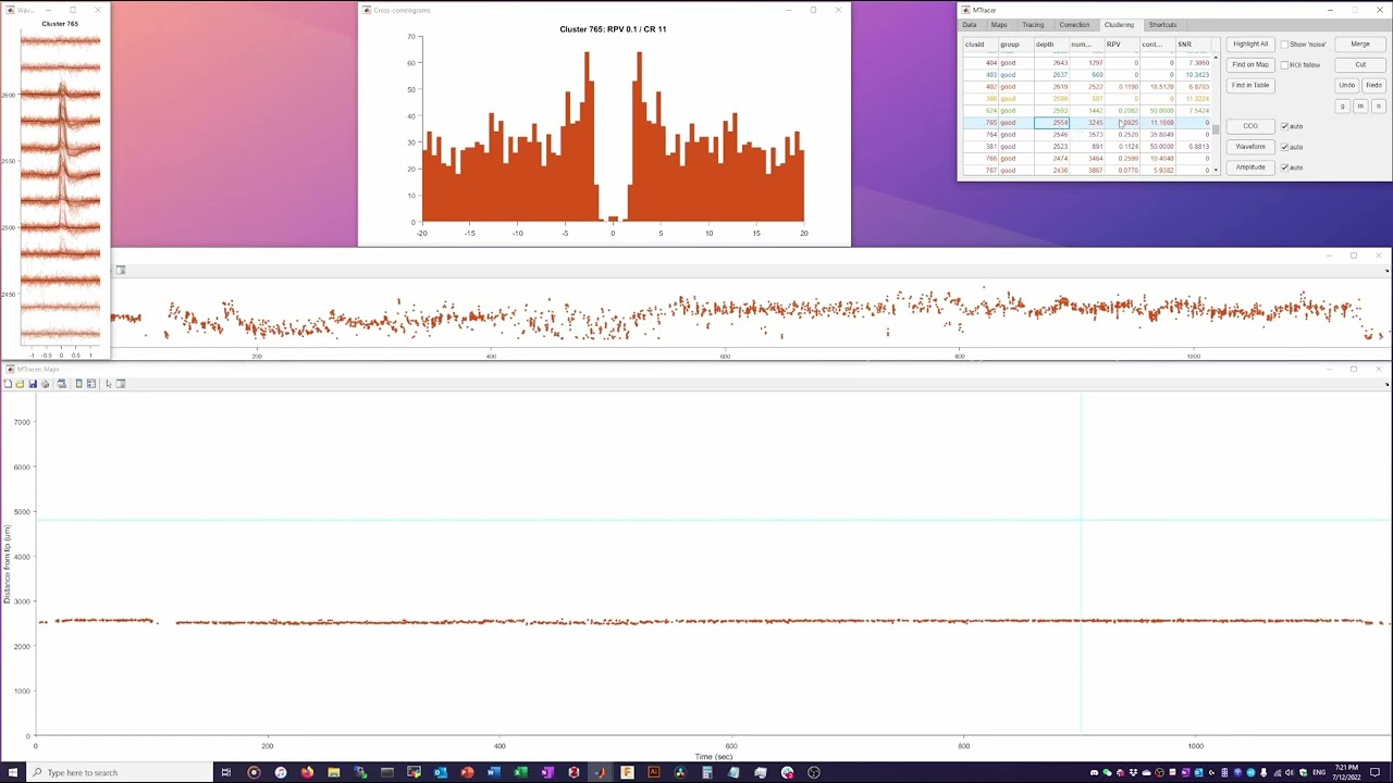
- Clustering Layer: Visualizes individual spikes as dots, colored by cluster membership.
The window supports three interaction modes:
- Navigation/Selection Mode: Change the focus point or select a nearby trace.
- Tracing Mode: Add anchor points to the tissue motion tracking traces.
- Cluster Cutting Mode: Cut spike clusters by drawing polygons.
Example Video 1: Drift Map Layer + Traces Layer (click to play on YouTube)
Example Video 2: Clustering Layer (click to play on YouTube)
Tabs
MTracer consists of several tabs, each serving a group of functions:
Data Tab
The Data tab allows you to load or link Neuropixels data:

Data Loading Fields:
- Channel Map: Path to the Neuropixels channel map file in .mat format
- ap.bin: Path to the raw AP (action potential) binary file
- AP data will not be read immediately, but is linked or mapped to memory.
- Snippets of AP traces can be plotted in Maps windows by pressing 'v' on the keyboard.
- lf.bin: Path to the raw LF (local field) binary file
- LF data will be read in full and downsample to 50 Hz for plotting as a heatmap.
- KS output dir: Path to the Kilosort output directory
- Load drift map: Import "drift map" if rez.mat is present.
- Load Phy: Load Phy-compatible Kilosort output, or an available cache file.
- Save Phy: Export clustering results back to Phy format.
- Save as cache: Cache clustering results to a .mat file for easier reuse.
Session Management:
- Recording Name: Set name for the current recording
- New Session: Start a fresh session
- Load Session: Restore a previous session
- Save Session: Save current session state
Maps Tab
The Maps tab contains the main visualization window and controls:

Maps Window:
- Open Maps: The main display showing multiple data layers. Supports pan, zoom, and various interaction modes
- Load Layout: Load a previously saved window layout
- Save Layout: Save the current window layout
AP Source:
- Choose between imec.ap.bin or temp_wh.dat for AP traces
Navigation:
- Focus: Showing/setting the time (in seconds) and depth (in μm) of the focus.
- Time Window: Showing/setting the time window (in seconds) to display.
- Depth Window: Showing/setting the depth window (in μm) to display.
- Remember: Remember the current time and depth window.
- Forget: Delete the selected time and depth window entry.
- Go to: Jump to a region of interest.
Layer Controls:
- Toggle visibility of different data layers:
- Focus indicator - Press '1'
- Drift map layer (raw spike positions) - Press '2'
- Clustering layer (cluster-colored spikes) - Press '3'
- AP traces layer - Press '4'
- LFP heatmap layer - Press '5'
- Anchor points - Press '6'
- Interpolated traces - Press '7'
Tracing Tab
The Tracing tab allows you to manage tissue movement tracking points:

Trace List:
- Displays list of traces with their timestamps and depths (e.g., "t: 0-32s, y: 2402um")
Trace Operations:
- Inspect: View details of selected trace such as a decomposition of slow drift and fast oscillations.
- Delete: Remove selected trace
- Merge: Combine multiple traces
- Load: Load previously saved traces
- Save: Save current traces as .mat files.
Auto Tracing:
- Tracer: Select tracking model.
- # points: Specify number of tracking points to generate
Correction Tab
The Correction tab allows you to apply drift correction to the data:

1) Load Interpolant: Load a previously saved interpolant derived from traces (using an external script).
2) Test with map data: Apply the interpolant to data in the Maps window for a preview.
3) Correct binaries: Apply the interpolant to the AP/LF data and save the corrected binaries.
Clustering Tab
The Clustering tab allows you to perform spike cluster curation:

The Clustering tab provides tools for manual curation of spike clusters:
Cluster List:
- Table showing cluster information
- Color-coded by cluster
- Click to select clusters for operations
Navigation and Visuals:
- Highlight All: Highlight all clusters
- Show Noise: Toggle visibility of noise clusters in gray
- Find on Map: Navigate to the location of selected clusters in the Maps window
- Find in Table: Selected the closest cluster to focus point in the table
- ROI follow: Toggle whether the ROI in Maps window follows the selected clusters
- Recolor: Reassign cluster colors
Cluster Operations:
- Merge: Combine selected clusters
- Cut: Enter polygon cutting mode to split clusters
- g/m/n: Label selected clusters as good/mua/noise
Feature Windows:
-
CCG (Cross-Correlogram): A grid of histograms showing the temporal relationship between spikes in different clusters.
- Diagonal histograms show the auto-correlogram of each cluster.
- Off-diagonal histograms show the cross-correlogram between each pair of clusters.
-
Waveform: Display spike waveforms from selected clusters. There are two ways of selection.
- Select from the cluster list.
- Select from the Maps window using MATLAB's brush tool.
-
Feature-time: Plots spike features over time. Press 'f' to cycle through the following features.
- Amplitude
- X-Position
Shortcuts Tab
In this tab, you can find documentation for all the shortcuts in the app.
| Category | Key | Function |
|---|---|---|
| Navigation | Click on map | Set focus |
| ] | Zoom in time | |
| [ | Zoom out time | |
| + | Zoom in depth | |
| - | Zoom out depth | |
| o | View the whole map | |
| c | Center focus | |
| w/s/a/d | Move up/down/left/right | |
| Shift + w/s/a/d | Move faster | |
| Scroll | Move left/right | |
| Plotting | 1 | Toggle focus indicator |
| 2 | Toggle raw spikes | |
| 3 | Toggle cluster spikes | |
| 4 | Toggle AP traces | |
| 5 | Toggle LFP heatmap | |
| 6 | Toggle anchor points | |
| 7 | Toggle interpolated traces | |
| . | Increase spike marker size | |
| , | Decrease spike marker size | |
| v | Plot AP traces around focus | |
| Tracing | t | Enter tracing mode |
| esc | Exit tracing mode | |
| Left click | Add an anchor point | |
| Right click | Undo selected point | |
| Ctrl + z | Undo last point | |
| Ctrl + Shift + z | Redo | |
| q | Query the next point with auto-tracer | |
| Clustering | k | Enter cluster cutting mode or confirm cut |
| esc | Cancel and exit cluster cutting | |
| Left click | Add a polygon vertex | |
| Right click | Remove last vertex | |
| Alt + g/m/n | Label selected cluster(s) good/mua/noise |
Support
For issues and feature requests, please use the GitHub issues page.